Excel For Mac Pivot Table Repeat Item Labels

This Excel tutorial explains how to create a pivot table in Excel 2011 for Mac (with screenshots and step-by-step instructions).

Rss bot for mac computer. See solution in other versions of Excel:

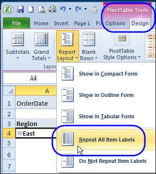
You can then select to Repeat All Item Labels which will fill in any gaps and allow you to take the data of the Pivot Table to a new location for further analysis. DOWNLOAD EXCEL WORKBOOK. Lego dc super villains demo. STEP 1: Click in the Pivot Table and choose PivotTable Tools Options (Excel 2010) or Design (Excel 2013 & 2016) Report Layouts Show in Outline/Tabular Form.

Question: How do I create a pivot table in Microsoft Excel 2011 for Mac?

Answer: In this example, the data for the pivot table resides on Sheet1.

Highlight the cell where you'd like to see the pivot table. In this example, we've selected cell A1 on Sheet2.

Next, select the Data tab from the toolbar at the top of the screen. Click on the PivotTable button and select Create Manual PivotTable from the popup menu.

A Create PivotTable window should appear. Select the range of data for the pivot table and click on the OK button. In this example, we've chosen cells A1 to D13 in Sheet1.

Next, select where you wish to place the PivotTable. In this example, we clicked on the 'Existing worksheet' option and set the location to Sheet2!$A$1.

Click on the OK button.

Your pivot table should now appear as follows:

In the PivotTable Builder window, choose the fields to add to the report. In this example, we've selected the checkboxes next to the Order ID and Quantity fields.

Next under the Values box, click on the 'Sum of Order ID' and drag it to the Row Labels box.

Your pivot table should now display the total quantity for each Order ID as follows:

Finally, we want the title in cell A2 to show as 'Order ID' instead of 'Row Labels'. To do this, select cell A2 and type Order ID.